I wanted to implement a simple neural network in C for quite a while now - artificial intelligence and deep learning are changing the world around us and although I’ve had a deep learning course at my university, it was quite theoretical and the exercises were mostly based on existing Python libraries. By working with C I get an opportunity to explore neural networks closer to hardware. Since I was exploring Wasimoff in parallel to this project, I decided to expand the scope and also execute the neural net on a distributed network of devices.
The goal of this project is to implement a dense neural network in C from scratch that can correctly recognise handwritten numbers and then deploy it with Wasimoff, a software enabling distributed computing by compiling programs in Web Assembly and then offloading these programs to browsers on available devices. The software is then to be tested on heterogeneous hardware (Raspberry Pi 4, e/OS/ smartphone, LineageOS tablet and an old Lubuntu machine).
The name of this project is HejmoNN, Hejmo is Esperanto for home.
The basics#
The perceptron#
The perceptron is the most basic neuron possible, it has several numerical imputs, which are each multiplied with a weight. If the sum of all products of weights and inputs is greater than a threshold the neuron outputs a one otherwise a zero.
$$ \text{output} = \begin{cases} 0 &\text{if } \sum_j w_j \cdot x_j \leq \text{threshold} \newline 1 &\text{if } \sum_j w_j \cdot x_j > \text{threshold} \end{cases} $$
We can introduce a bias \(b\) to simplify the notation (the bias is just a number that tells us how easily a threshold can be reached, in fact it is equal to \(-\text{threshold}\)):
$$ \text{output} = \begin{cases} 0 &\text{if } \sum_j w_j \cdot x_j + b \leq 0 \newline 1 &\text{if } \sum_j w_j \cdot x_j + b > 0 \end{cases} $$
These neurons can be connected together to form a mesh where the first layer of neurons processes external inputs and gives the result to the second layer before the final layer makes a binary decision like in this case:
This is in fact how the first neural networks in early animals worked - we can still see the early stages of simple neural networks in jellyfish where the nerves form a net and a ring - the jellyfish responds to a small set of inputs (such as external presure, temperature) and transforms these inputs into a small set of possible outputs (such as to swim or not to swim) - except that the thresholds in animals are regulated by electrochemical potentials instead of digital values.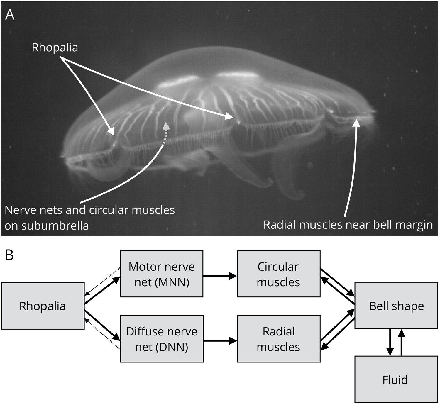
Perceptrons can compute basic computational functions like AND, OR and NAND. Networks of perceptrons can be used to implement any logic function - so theoretically one could also build a computer out of neurons 🤠.
However unlike logic gates which cannot change and must be designed explicitly, neurons can be trained to change weights in order to solve a problem without modifying the circuit.
The Sigmoid neuron#
Sigmoid neurons work similar to the perceptron, but the inputs can be any number between 0 and 1 and the output is also between 0 and 1 as specificied by the sigmoid function:
$$ \text{output} = \frac{1}{1+e^{\sum_j w_j \cdot x_j - b}} $$
The sigmoid output function is continuous and smooth unlike the perceptron’s output, so a small change in the weights and the bias produces a small change in the output of the neuron:
$$ \Delta\text{output} \approx \sum_j \frac{\partial \text{output}}{\partial w_j} \Delta w_j + \frac{\partial \text{output}}{\partial b} \Delta b$$
Layers of neurons that are not inputs or output neurons are called hidden layers, though the name is a bit misleading, since they aren’t actually hidden.
If we wanted to determine whether a 64x64 image is a nine then we’d need 4096 inputs (or alternatively we could use a convolutional neural network) and the output layer would only have one neuron, where if the output would be greater than 0.5 we’d say that we have a 9 and if it were less than that we’d say we don’t have a nine. The number of hidden neurons and layers is largely a question of heuristics.
Simple network for digit classification#
I’m aiming for something like this:
A neural network which can recognise which digit is present on a given input image (where each image has 28x28 greyscale pixels). The neuron with the highest output value is equal to the digit in the picture. I will be using the MINST data set
The desired output \(y(x)\) for a given input \(x=6\) is then the vector: $$y(x)=\begin{pmatrix} 0 \newline 0 \newline 0 \newline 0 \newline 0 \newline 0 \newline 1 \newline 0 \newline 0 \newline 0 \newline \end{pmatrix}$$
We need to define a metric to see how well our system determines the output - this can be done with a cost function:
$$C(w, b) = \frac{1}{2n} \sum_x ||y(x)-a||^2$$
Where \(w\) are the weights, \(b\) the biases, \(n\) is the number of training inputs, \(a\) is the vector of outputs when \(x\) is input, and \(y(x)\) is the correct solution. \(||x||\) is the norm of \(x\) which is typically the mean square error:
$$MSE= \frac{1}{n}\sum_{i=1}^n (y_i- \hat{y}_i)^2$$
Obviously we wish to minimise the cost function, but how can we do so? The answer is to use the gradient descent in order to find the (hopefully global) minimum of the multidimensional function. The gradient of the cost or error function, \(C\), is equal to:
$$\nabla C(w, b) = \begin{pmatrix} \frac{\partial C(w,b)}{\partial w} & \frac{\partial C(w,b)}{\partial b} \end{pmatrix}^T$$
and we can write \(\Delta C(v)\) as \(\Delta C(v) \approx \nabla C(v) \cdot \Delta v\). If we choose \(\Delta v = - \eta \nabla C(v)\) where \(\eta\) is a small number refered to as the learning rate and is ideally equal to \(\eta = \frac{||\Delta v||}{\nabla C(v)} \). Since \(||\nabla C(v)||^2 \geq 0\), the equation \(\Delta C(v) \approx -\eta ||\nabla C(v)||^2\) will always be smaller than 0 - so the error, \(C(v)\), will decrease. So we can construct the rule:
$$w_{\text{new}}=w-\eta \frac{\partial C}{\partial w}$$ $$b_{\text{new}}=b-\eta \frac{\partial C}{\partial b}$$
Sadly calculating all derivatives with Newton’s method can be too costly, just because of the sheer number of weights.
In order to efficiently compute the gradient, we can simply compute a small sample of randomly chosen training inputs - averaging over this sample gives a pretty good estimate - this is called the stochastic gradient descent:
$$w_{\text{new}}=w-\frac{\eta}{m} \sum^m \frac{\partial C}{\partial w}$$ $$b_{\text{new}}=b-\frac{\eta}{m} \sum^m \frac{\partial C}{\partial b}$$
A great visualisation of everything I summarise here is available in this video:
The implementation#
This implementation is based on the theory of stochastic gradient descent and backpropagation from Nielsen’s book and Gajdus’ implementations of neural networks in C - I will also stick to Gajdus’ explanation of the backpropagation algorithm with inspirations from Mayur Bhole’s implementation sprinkled here and there.
Loading the MNIST Dataset#
One of the first challenges is to actually correctly read the MNIST dataset - since we’re working with C we have to know how the data is structured. The training images are available in a .idx3-ubyte-format. The data is stored in the following format:
magic number
size in dimension 0
size in dimension 1
size in dimension 2
.....
size in dimension N
data
The magic number (and the data) is written in the MSB format and tells us if we deal with a image or label dataset. The third byte tells us what kind of data we’re dealing with:
0x08: unsigned byte
0x09: signed byte
0x0B: short (2 bytes)
0x0C: int (4 bytes)
0x0D: float (4 bytes)
0x0E: double (8 bytes)
The 4-th byte codes the number of dimensions of the vector/matrix: 1 for vectors, 2 for matrices…. The sizes in each dimension are 4-byte integers (MSB first, high endian, like in most non-Intel processors). The data is stored like in a C array, i.e. the index in the last dimension changes the fastest.
The only standard headers we’ll be working with (for now) will be:
#include <stdio.h> // for reading and printing outputs
#include <stdlib.h> // for malloc
Since Intel/AMD processors are LSB first we first need to convert the integers from their MSB form into their LSB counterparts:
unsigned int reverseBytes(unsigned int num) {
    return ((num >> 24) & 0x000000FF) |
           ((num >> 8) & 0x0000FF00) |
           ((num << 8) & 0x00FF0000) |
           ((num << 24) & 0xFF000000);
}
I’ll be saving the images as 1-byte arrays:
int main {
   int numImg;
   int imgSize;
   unsigned char** img;
   return 0;
}
I printed the first image to test if everything works. I decided to use PPM for this purpose - this is the same image format that I’ve already used in my Raytracing adventure.
This way we don’t need any special headers or libraries and at least on Linux PPM-images are readable by default.
void toPPM(const char* filename, unsigned char* img, int width, int height) {
    FILE* file = fopen(filename, "w");
    if (!file) {
        printf("Couldn't open %s\n", filename);
        return;
    }

    fprintf(file, "P3\n");
    fprintf(file, "%d %d\n", width, height);
    fprintf(file, "255\n");

    for (int i = 0; i < height; i++) {
        for (int j = 0; j < width; j++) {
            unsigned char pixel = img[i * width + j];
            // since we're working with greyscale it holds that R=G=B
            fprintf(file, "%d %d %d ", pixel, pixel, pixel);
        }
        fprintf(file, "\n");
    }

    fclose(file);
}
Next up is the actual reading of the dataset and saving it in a dynamically allocated array. First we’ll be opening the file containing the data, then check the magic number (it should be 2051 for the image dataset), the number of images, rows, columns, and finally we load the images:
unsigned char** loadImg(const char* filename, int* numImg, int* imgSize) {
    FILE* file = fopen(filename, "rb");
    if (!file) {
        printf("Couldn't open %s\n", filename);
        return NULL;
    }

    unsigned int magicNumber, nItems, nRows, nCols;
    fread(&magicNumber, sizeof(unsigned int), 1, file);
    magicNumber = reverseBytes(magicNumber);
    if (magicNumber != 2051) {
        printf("Invalid magic number\n");
        fclose(file);
        return NULL;
    }

    fread(&nItems, sizeof(unsigned int), 1, file);
    *numImg = reverseBytes(nItems);
    fread(&nRows, sizeof(unsigned int), 1, file);
    fread(&nCols, sizeof(unsigned int), 1, file);
    *imgSize = reverseBytes(nRows) * reverseBytes(nCols);

    unsigned char** img = (unsigned char**)malloc(*numImg * sizeof(unsigned char*));
    for (int i = 0; i < *numImg; i++) {
        img[i] = (unsigned char*)malloc(*imgSize * sizeof(unsigned char));
        fread(img[i], sizeof(unsigned char), *imgSize, file);
    }

    fclose(file);
    return img;
}
I can now finalise the main function:
int main(void) {
   int numImg;
   int imgSize;
   unsigned char** img = = loadImg("train-images-idx3-ubyte", &numImg, &imgSize);

   toPPM("first_image.ppm", img[0], 28, 28);

   for (int i = 0; i < numImg; i++) {
      free(img[i]);
   }
   free(img);
   return 0;
}
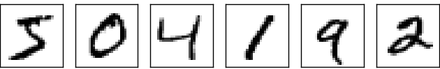
And it works! The first two images are:


The next step is to read out the correct image label values, which are also provided by NIST. The magic number for the label set is 2049.
unsigned char* loadLabels(const char* filename, int* numLabels) {
    FILE* file = fopen(filename, "rb");
    if (!file) {
        printf("Couldn't open %s\n", filename);
        return NULL;
    }

    unsigned int magicNumber, nItems;
    fread(&magicNumber, sizeof(unsigned int), 1, file);
    magicNumber = reverseBytes(magicNumber);
    if (magicNumber != 2049) {
        printf("Invalid magic number\n");
        fclose(file);
        return NULL;
    }

    fread(&nItems, sizeof(unsigned int), 1, file);
    *numLabels = reverseBytes(nItems);

    unsigned char* labels = (unsigned char*)malloc(*numLabels * sizeof(unsigned char));
    fread(labels, sizeof(unsigned char), *numLabels, file);

    fclose(file);
    return labels;
}
Giving the new main function:
int main(void) {
    int numImg;
    int imgSize;
    unsigned char** img = loadImg("train-images.idx3-ubyte", &numImg, &imgSize);
    int numLabels;
    unsigned char* labels = loadLabels("train-labels.idx1-ubyte", &numLabels);

    toPPM("first_image.ppm", img[0], 28, 28);
    printf("The labels are %u, %u\n", labels[0], labels[1]);

    for (int i = 0; i < numImg; i++) {
       free(img[i]);
    }
    free(img);
    return 0;
 }
And we get 5 and 0, just as expected! Now we can start programming the actual neural network. All of this could easily be done with a few Python functions, so it’s no surprise Python and R are so dominant in data science.
Architecture of the neural network#
To start off, I’ll create two structs. The first one is called layer:
typedef struct layer {
    float *weights, *biases;
    int numInputs, numNeuro;
} layer;
The layer-struct represents the layer which will contain the neurons - it tells us how many neurons are in the layer, how many inputs each neuron has, as well as the weights and biases of each neuron.
After that I’ll create network:
typedef struct network {
    layer *hidden, *output;
} network;
The struct will contain the layers of our DNN with the exception of the input layer, because it’s trivial.
Next the layers, weights and neurons need to be inititalised. I’ll create \(28^2\) nerons in the input layer, 15 neurons in the hidden layer and of course 10 neurons in the output layer. Just in case we want to change the number of hidden neurons I’ll add the following macro:
#define HIDDEN 15
Just like in Gajdus’ implementation the biases will be initialised as zeroes, but for the weights I will be using the Xavier initalisation, which keeps the scale of the gradients roughly similar in all layers, preventing the gradients from exploding or vanishing during the learning phase when used with sigmoid functions. For \(n_{in}\) inputs and \(n_{out}\) we can define the uniform Xavier intialisation as:
$$ W \sim \mathcal{U}(- \sqrt{\frac{6}{n_{in}+n_{out}}}, \sqrt{\frac{6}{n_{in}+n_{out}}}) $$
The only functions I’d be needing from math.h would be the square root and the exponential function, so I decided to implement both myself and not import any extra libraries. To compute the square I’ll use Heron’s Method from ancient Greece. Let \(A\) and \(x_0\) be positive real numbers, where \(A\) is the number whose square we are looking forand \(x_0\) a random initial guess, then we can perform an iteration utill we aren’t satisfied with the accuracy like this:
$$ \sqrt{x} = \lim_{i \rightarrow \infty} x_i = \frac{x_{i-1}+\frac{A}{x_{i-1}}}{2}$$
float sqr(float x) {
    float x_new = x / 2.0;
    float epsilon = 0.1;
    float prev_x;

    while (prev_x - x_new > epsilon || prev_x- x_new < -epsilon) {
        prev_x = x_new;
        x_new = 0.5 * (x_new + x / x_new);
    }
    return x_new;
}
This gives the following code to initialise all the layers and neurons:
void init_layer(struct layer *layer, int numInputs, int numNeurons) {
    srand(42);
    int n = numInputs * numNeurons;
    float xavier = sqr(6.0 / ((float)numNeurons + (float)numInputs));

    layer->numInputs = numInputs;
    layer->numNeuro = numNeurons;
    layer->weights = malloc(n * sizeof(float));
    layer->biases = malloc(numNeurons * sizeof(float));


    for (int i = 0; i < n; i++) {
        layer->weights[i] = ((float)rand() / RAND_MAX - 0.5) * xavier;
    }

    for (int i = 0; i < numNeurons; i++) {
        layer->biases[i] = 0;
    }

}
Preparing the forward pass#
To prepare the forward pass one has to first implement the exponential function. The forward pass is simply the calculation of an output for a given input image. We’ll use the taylor series of degree 3 (which yields a minimal error within \([-1,1]\)) and restrict ourselves to floats (doubles will give us more accuracy, but I aim for memory efficiency):
$$e^x = \sum_{n=0}^{\infty} \frac{x^n}{n!}\approx 1 + x + \frac{x^2}{2}+\frac{x^3}{6}$$
float e(float x) {
    return 1.0 + x + x*x/2.0 + x*x*x/6.0;
}
We now define the sigmod function:
float sigmoid(float x) {
    return 1.0 / (1.0 + e(-x));
}
The function has a pretty neat derivative, let \(S(x)\) be the sigmoid function, then the derivative is equal to:
$$S’(x) = S(x)(1-S(x))$$
To implement the feed-forward function we need to apply the equation:
$$\textit{a}^i_j = \sigma(\sum_k \textit{w}^i_{jk} \cdot a_k^{i-1}+ b_j^i)$$
In this equation \(a\) is the activation, \(w\) are the outgoing weights, \(b\) are the biases, \(i\) represents the layer, and \(j\) is the neuron number. This is in line with the notation from the visualisation below:
In the feedforward function we also divide the input by 256 to ensure it is normalised (this will make sure that my values are compatible with the Sigmoid function):
void normalize_input(float *input) {
    for (int i = 0; i < 784; i++) {
        input[i] /= 255.0;
    }
}
and now the feedforward function itself:
void forward_prop(struct layer *layer, float *input, float *output) {
    for (int i = 0; i < layer->numNeuro; i++)
        output[i] = layer->biases[i];

        for (int j = 0; j < layer->numInputs; j++) {
            for (int i = 0; i < layer->numNeuro; i++) {
                output[i] += input[j] * layer->weights[j * layer->numNeuro + i];
            }
        }

    for (int i = 0; i < layer->numNeuro; i++) {
        output[i] = sigmoid(output[i]);
    }
}
Preparing the backward pass#
The backward pass will update the weights to minimise the mean squared error (as defined above).
In order to implement the backwards propagation, we first define the weighted input quantity \(z^l = w^l a^{l-1}+b^l\). This quantity allows us to define the error of neuron j in layer l with:
$$\delta^l_{j} = \frac{\partial C}{\partial z^l_j}$$
Using this definition it is possible to build backpropagation on four basic equations - I will be sticking to Gajdus’ form of the equations. The first one is the weight update formula (1):
$$w_{ij}=w_{ij}-\eta \cdot \frac{\partial C}{\partial w_{ij}}$$
The weight update subtracts the gradient of the loss function with respect to the individual weight. Next up is the bias update formula (2):
$$b_i=b_i-\eta \cdot \frac{\partial C}{\partial b_{i}}$$
The bias is updated in a similar manner, but the gradient of the loss function with respect to the invidual neuronal bias is used. The input gradient is calculated as (3):
$$\frac{\partial C}{\partial x_j}=\sum_{i=1}^n \frac{\partial C}{\partial y_i} \cdot w_{ij}$$
The partial derivative of the loss function with respect to the input \(x_j\) is computed as the sum of the products of the partial derivatives of the loss with respect to each output \(y_i\) and their corresponding weights \(w_{ij}\). The gradient for the weights is calculated as follows (4):
$$\frac{\partial C}{\partial w_{ij}}=\frac{\partial C}{\partial y_i} \cdot x_{j}$$
This all gives the following code for the backpropagation pass of multiple desired outputs.
void back_prop(struct layer *layer, float *input, float *output_grad, float *input_grad, float eta) {
    for (int i = 0; i < layer->numNeuro; i++) {
        for (int j = 0; j < layer->numInputs; j++) {
            int idx = j * layer->numNeuro + i;
            float grad = output_grad[i] * input[j]; // Eq 4
            layer->weights[idx] -= eta * grad; // Eq 1
            if (input_grad != NULL) {
                input_grad[j] += output_grad[i] * layer->weights[idx]; // Eq 3
            }
        }
        layer->biases[i] -= eta * output_grad[i]; // Eq 2
    }
}
Training#
The training combines both forward and backward passes; We first send a image through the network and then check how big the error is - using this information we can then use backpropagation to prepare a good estimate for how much the weights and biases need to be changed.
For the training parameters I will introduce the macro definitions:
#define ETA 0.001
#define EPOCHS 3
We will pick a learning rate, η, of 0.001 and three epochs.
Neural networks are typically trained using several epochs - an epoch is a complete pass through the entire training set. In addition to that batches are typically used to speed up the training process - a batch is a number of training samples that are run through the model before the weights are updated. The reason behind using batches is to speed up the learning process - but batches won’t be used in this implementation.
void training(struct network *net, float *input, int label, float eta) {
    float hidden_output[HIDDEN] = {0}, final_output[10] = {0};
    float hidden_grad[HIDDEN] = {0}, output_grad[10] = {0};
    float target[10] = {0};

    target[label] = 1.0;

    forward_prop(net->hidden, input, hidden_output);
    forward_prop(net->output, hidden_output, final_output);
    for (int i = 0; i < 10; i++) {
        output_grad[i] = final_output[i] - target[i];
    }

    back_prop(net->output, hidden_output, output_grad, hidden_grad, eta);
    for (int i = 0; i < HIDDEN; i++) {
        hidden_grad[i] *= sigmoid(hidden_output[i]) * (1-sigmoid(hidden_output[i]));
    }
    back_prop(net->hidden, input, hidden_grad, NULL, eta);
}

void train(struct network *net, unsigned char** img, unsigned char* labels, int numImg) {
    float input[28 * 28];
    for (int epoch = 1; epoch < EPOCHS+1; epoch++) {
        for (int i = 0; i < numImg; i++) {
            for (int j = 0; j < 28 * 28; j++) {
                input[j] = (float)img[i][j] / 255.0;
            }
            training(net, input, (int)labels[i], ETA);
        }
        printf("Epoch %d done\n", epoch);
    }
}
Two more functions are now needed: A function to predict the digit of the input image and an evaluation function that tells us how well the model is performing.
To find the prediction we will have to take a look at the values at the output neurons - the neurons in a way measure the probability that a certain digit is present on the image and every output neuron will have a certain float value:
- Neuron 0: Probability digit we have a zero is: 0.001
- Neuron 1: Probability digit we have a one is: 0.032
- Neuron 2: Probability digit we have a two is: 0.891
The predicted digit is simply the neuron number with the highest probability - in the example above the digit is highly likely a two 🤠.
int predict(struct network *net, float *input) {
    float hidden_output[HIDDEN] = {0}, final_output[10] = {0};

    forward_prop(net->hidden, input, hidden_output);
    forward_prop(net->output, hidden_output, final_output);

    int max = 0;

    for (int i = 0; i < 10; i++) {
        if (final_output[i] > final_output[max]) {
            max = i;
        }
    }
    return max;
}

float evaluate(struct network *net, unsigned char** img, unsigned char* labels, int numImg) {
    float input[28 * 28];
    int correct = 0;
    for (int i = 0; i < numImg; i++) {
        for (int j = 0; j < 28 * 28; j++) {
            input[j] = (float)img[i][j] / 255.0;
            //printf("Input[%d]=%f\n", j, input[j]);
        }

        int label = labels[i];
        int prediction = predict(net, input);
        //printf("Predicted digit: %d\tActual digit: %d\n", prediction, label);

        if (prediction == label) {
            correct++;
        }
    }
    return (float) correct / (float) numImg * 100.0;
}
Excellent! All that is left is to rewrite the main function which incorporates all the code that implements the neural network.
int main(void) {
    int numImg;
    int imgSize;
    unsigned char** img = loadImg("train-images.idx3-ubyte", &numImg, &imgSize);
    int numLabels;
    unsigned char* labels = loadLabels("train-labels.idx1-ubyte", &numLabels);

    //toPPM("first_image.ppm", img[0], 28, 28);
    //printf("The labels are %u, %u\n", labels[0], labels[1]);

    if (numImg != numLabels) {
        printf("Mismatch between number of images and labels!\n");
        return 1;
    }

    network *homeNN = (network*)malloc(sizeof(network));
    layer *hidden = (layer*)malloc(sizeof(layer));
    layer *output = (layer*)malloc(sizeof(layer));
    homeNN->hidden = hidden;
    homeNN->output = output;
    init_layer(hidden, 28*28, HIDDEN);
    init_layer(output, HIDDEN, 10);

    train(homeNN, img, labels, 1000);

    printf("The accuracy is %f %%\n", evaluate(homeNN, &img[1000], &labels[1000], 1000));

    free_architecture(homeNN);

    for (int i = 0; i < numImg; i++) {
        free(img[i]);
    }
    free(img);
    free(labels);

    return 0;
}
In case you’re wondering, free_architecture() simply deallocates all the dynamically allocated memory - it is necessary for memory safety 🦺!
void free_architecture(struct network *net) {
    if (net->hidden->weights != NULL) {
        free(net->hidden->weights);
    } if (net->hidden->biases != NULL) {
        free(net->hidden->biases);
    } if (net->output->weights != NULL) {
        free(net->output->weights);
    } if (net->output->biases != NULL) {
        free(net->output->biases);
    }

    free(net->hidden);
    free(net->output);
    free(net);
}
And now we compile with gcc -o homeNN main.c and run the program ./homeNN (I set the number of training images to 1000 and the number of evaluation images to 1000) and:
The accuracy is 9.400000 %
Ha ha 😅 that’s worse than randomly picking an answer! Sadly simply increasing the number of training images made the result even worse, giving me an accuracy of 9.25% when evaluated with 2000 images 🫣.
Alright, I’ve set the learning rate to 0.01 and since we have 60 000 images, I’ve decided to split the entire set 80:20 - so the first 80% of the images will be used to train the neural network. Sadly however the predict() function always returns 0. Here’s what the outputs of the individual neurons were like:
Hidden Neuron 0 contains: 0.000000
Hidden Neuron 1 contains: 0.000000
Hidden Neuron 2 contains: 0.000000
Hidden Neuron 3 contains: 0.000000
Hidden Neuron 4 contains: -0.000000
Hidden Neuron 5 contains: -0.000000
Hidden Neuron 6 contains: -0.000000
Hidden Neuron 7 contains: -0.000000
Hidden Neuron 8 contains: 0.000000
Hidden Neuron 9 contains: -0.000000
Hidden Neuron 10 contains: -0.000000
Hidden Neuron 11 contains: -0.000000
Hidden Neuron 12 contains: -0.000000
Hidden Neuron 13 contains: 0.000000
Hidden Neuron 14 contains: 0.000000

Output Neuron 0 contains: 0.126749
Output Neuron 1 contains: 0.099787
Output Neuron 2 contains: 0.103147
Output Neuron 3 contains: 0.097592
Output Neuron 4 contains: 0.076131
Output Neuron 5 contains: 0.075863
Output Neuron 6 contains: 0.097544
Output Neuron 7 contains: 0.108539
Output Neuron 8 contains: 0.117372
Output Neuron 9 contains: 0.095782
Predicted digit: 0	Actual digit: 3


Hidden Neuron 0 contains: 0.000000
Hidden Neuron 1 contains: 0.000000
Hidden Neuron 2 contains: 0.000000
Hidden Neuron 3 contains: -0.000000
Hidden Neuron 4 contains: -0.000000
Hidden Neuron 5 contains: -0.000000
Hidden Neuron 6 contains: 0.000000
Hidden Neuron 7 contains: -0.000000
Hidden Neuron 8 contains: 0.000000
Hidden Neuron 9 contains: -0.000005
Hidden Neuron 10 contains: -0.000000
Hidden Neuron 11 contains: -0.000000
Hidden Neuron 12 contains: -0.000000
Hidden Neuron 13 contains: 0.000000
Hidden Neuron 14 contains: 0.000000

Output Neuron 0 contains: 0.126749
Output Neuron 1 contains: 0.099787
Output Neuron 2 contains: 0.103148
Output Neuron 3 contains: 0.097591
Output Neuron 4 contains: 0.076131
Output Neuron 5 contains: 0.075864
Output Neuron 6 contains: 0.097544
Output Neuron 7 contains: 0.108538
Output Neuron 8 contains: 0.117372
Output Neuron 9 contains: 0.095781

Predicted digit: 0	Actual digit: 8
Aha! Looks like the output neurons are all so close for every input because the outputs of the hidden neurons are simply too small! One thing worth trying at this point would be to use more hidden neurons or to use a different activation function, but after consulting Le Chat I decided to give the higher accuracy of math.h a try, so I implemented some changes, I added the standard maths library:
#include <math.h>
and stopped using sqr() and e():
float xavier = sqrt(6.0 / ((float)numNeurons + (float)numInputs));
float sigmoid(float x) {
    return 1.0 / (1.0 + exp(-x));
}
and now BAM! I get:
The accuracy is 81.800003 %
I decided to increase the number of hidden neurons to 64, and use 48000 images for the training and 12000 for the evaluation, which resulted in an accuracy of 86 %. I then also decided to see how the accuracy changes over epochs at different learning rates, η, and this is what I’ve observed:
This graph goes to show that even greater accuracies can be achieved at a lower η. According to Nielsen he reached a peak with the stochastic gradient descent at epoch 28 equalling to 95.42% (though with a η of 3.0), Gajdus who used ReLUs and Softmax activation functions managed to reach 98.22% - the best accuracy I managed to score was 92.67% at η equal to 0.001 after 20 epochs - but I’m satisfied with anything above 90% 😊. Interesting an η of 0.1 was just too big and the accuracy would not change fom 9.97%.
Preparing the model for a distributed execution#
Excellent, now that the model works, I need to prepare it for a distributed execution. The first thing I will do is better organise the file structure of the project:
HejmoNN/
│
├── src/
│   ├── nn.c                    # Main neural network (everything up to now)
│   ├── training.c              # Neural network training implementation
│   └── client.c                # Client-side implementation
│
├── include/
│   ├── cJSON.c              # cJSON Library
│   └── cJSON.h                 # cJSON Library
│
├── data/
│   ├── train-images.idx3-ubyte # Example image file
│   ├── train-labels.idx1-ubyte # Example image file
│   └── first_image.ppm         # First image generated
│
├── build/                      # Directory for build artifacts
│
├── README.md                   # Project overview and instructions
└── LICENSE                     # License information
One of the first things I’ll do is import cJSON, which will allow us to work with JSON files (at least on Linux I had to download the source, and place the cJSON.c and cJSON.h in the include folder):
#include "cJSON.h"
The compilation will be done like this:
gcc -o build/train src/train.c include/cJSON.c -Iinclude -lm
Excellent, now we can create a function that will export the sizes of each layer and the individual weights and biases to a JSON file:
void export_layer_to_json(cJSON *root, const char *layer_name, struct layer *layer) {
    cJSON *layer_obj = cJSON_CreateObject();

    cJSON_AddNumberToObject(layer_obj, "numInputs", layer->numInputs);
    cJSON_AddNumberToObject(layer_obj, "numNeuro", layer->numNeuro);

    cJSON *weights_array = cJSON_AddArrayToObject(layer_obj, "weights");
    cJSON *biases_array = cJSON_AddArrayToObject(layer_obj, "biases");

    for (int i = 0; i < layer->numInputs * layer->numNeuro; i++) {
        cJSON_AddItemToArray(weights_array, cJSON_CreateNumber(layer->weights[i]));
    }

    for (int i = 0; i < layer->numNeuro; i++) {
        cJSON_AddItemToArray(biases_array, cJSON_CreateNumber(layer->biases[i]));
    }

    cJSON_AddItemToObject(root, layer_name, layer_obj);
}

void export_network_to_json(const char* filename, struct network *net) {
    cJSON *root = cJSON_CreateObject();

    export_layer_to_json(root, "hidden_layer", net->hidden);
    export_layer_to_json(root, "output_layer", net->output);

    FILE *file = fopen(filename, "w");
    if (file == NULL) {
        printf("Couldn't open %s\n", filename);
        cJSON_Delete(root);
        return;
    }

    char *json_string = cJSON_Print(root);
    fprintf(file, "%s", json_string);
    free(json_string);
    fclose(file);

    cJSON_Delete(root);
}
What is being done here is the following: first we save the number of inputs and neurons in each layer, which correspond to our layer struct then we write the weights and biases and simply repeat the same process for the output layer - the whole data will be exported to network.json - it will look something like this:
{
        "hidden_layer": {
                "numInputs":    784,
                "numNeuro":     64,
                "weights":      [-0.039242561906576157, -0.014302699826657772, ...
                "biases":       [-0.052776895463466644, 0.22721207141876221, ...
        },
        "output_layer": {
                "numInputs":    64,
                "numNeuro":     10,
                "weights":      [-1.1562167406082153, -0.22629979252815247, ...
                "biases":       [-0.527853488922119, -0.19712990522384644, ...
        }
}
At just a mere 64 hidden neurons I have 1,1 MB worth of model data. If this model were to be used in an embedded context, I would highly recommend quantisation, which would reduce the model size by a factor of 4 - in fact we have to save \(n \cdot (784 + 10)\) weights and \(n + 10\) biases (if \(n\) is the number of hidden neurons).
Excellent! Now the data needs to be imported - this will be done in the client.c file.
void import_layer_from_json(cJSON *layer_obj, struct layer *layer) {
    cJSON *weights_array = cJSON_GetObjectItem(layer_obj, "weights");
    cJSON *biases_array = cJSON_GetObjectItem(layer_obj, "biases");

    layer->numInputs = cJSON_GetObjectItem(layer_obj, "numInputs")->valueint;
    layer->numNeuro = cJSON_GetObjectItem(layer_obj, "numNeuro")->valueint;

    int n = layer->numInputs * layer->numNeuro;
    layer->weights = (float*)malloc(n * sizeof(float));
    layer->biases = (float*)malloc(layer->numNeuro * sizeof(float));

    for (int i = 0; i < n; i++) {
        layer->weights[i] = cJSON_GetArrayItem(weights_array, i)->valuedouble;
    }

    for (int i = 0; i < layer->numNeuro; i++) {
        layer->biases[i] = cJSON_GetArrayItem(biases_array, i)->valuedouble;
    }
}

void import_network_from_json(const char* filename, struct network *net) {
    FILE *file = fopen(filename, "r");
    if (file == NULL) {
        printf("Couldn't open %s\n", filename);
        return;
    }

    fseek(file, 0, SEEK_END);
    long length = ftell(file);
    fseek(file, 0, SEEK_SET);
    char *json_data = (char*)malloc(length + 1);
    fread(json_data, 1, length, file);
    fclose(file);
    json_data[length] = 0;

    cJSON *root = cJSON_Parse(json_data);
    free(json_data);

    if (root == NULL) {
        printf("Error parsing JSON\n");
        return;
    }

    cJSON *hidden_layer_obj = cJSON_GetObjectItem(root, "hidden_layer");
    cJSON *output_layer_obj = cJSON_GetObjectItem(root, "output_layer");

    net->hidden = (struct layer*)malloc(sizeof(struct layer));
    net->output = (struct layer*)malloc(sizeof(struct layer));

    import_layer_from_json(hidden_layer_obj, net->hidden);
    import_layer_from_json(output_layer_obj, net->output);

    cJSON_Delete(root);
}
The import and the evaluation work as a charm! This way we can now train models on powerful machines, offload the code, import the models quickly and then perform calculations on less powerful remote devices in our network.
Distributed computing: Wasimoff#
In the past many scientific problems were solved using distributed computing - tasks would be split among many computers on a network. One of the most remarkable examples of this is volunteer computing. Folding@Home is one of such projects which simply used the idle computing power of its volunteers - most notably utilising the PS3’s GPU, when people weren’t playing. There are also other examples of distributed computing - the most well known one being cloud computing
Distributed computing is thus quite useful - we could use a set of devices in our own network and simply split a large data set among the devices for processing. But how can one do so? The practical answer is by using middleware. The Folding@Home project used BOINC - BOINC would send the software necessary to the volunteer client, who would perform the calculations and then send the result back to the server, but BOINC has one big drawback: software needs to be compiled for every hardware architecture (x86 32-bit and 64-bit, ARM, RISC-V), every operating systems and GPU separately.
And this is where Wasimoff comes into play. It is similar to BOINC in the sense that it offloads code to other devices, but it enables us to offload the code to any device regardless of the computer architecture - we do so by compiling the programme using WebAssembly and then run the program on all the devices simply in the browser. WebAssembly is a binary instruction format - it allows us to compile C/C++ programs into WebAssembly and then execute them on Firefox or Chrome.
In Wasimoff we have three roles:
- The Broker which is the computer coordinating all the offloading.
- The Provider which is a computer that executes the code for others
- The Client which uploads programs and computational tasks.
First and foremost we have to download Wasimoff:
git clone https://github.com/wasimoff/wasimoff.git
Then we need to start the broker in a docker container. First we need to go to the webprovider folder and run:
yarn build
This command will build the Webprovider, which is the website that our provdiers can connect to. Then we need to go to the root folder of Wasimoff and run:
sudo docker build --target wasimoff -t wasimoff:broker .
and the broker can be started with:
sudo docker compose up broker
or you can simply run the following if you wish to start both the broker, webprovider page and a provider on the machine this code is run on (if you’re unsure it’s best to run this):
sudo docker compose up
sudo docker ps and stop them sudo docker stop <id> - but if you do so don’t forget to remove any unnecessary leftover files: sudo docker system prune -a freed up 33 GB of memory on my system!And here we go - our middleware is all setup: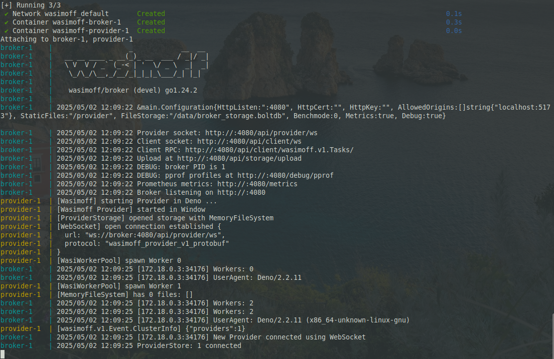
To open the locally hosted Wasimoff website we simply have to go to http://localhost:4080 or to http://<ip-address-of-your-computer>:4080 on other devices:

http site and not the https site.Other devices simply need to open the website to become the providers.
Next up we need to compile our C-program into webassembly so it can be offloaded to providers. To do so we need a Webassembly compiler - I’ll simply stick to emscripten. Luckily on Linux Mint it’s very easy to install it from the software manager, on other platforms you can find the instructions here.
It’s very important that we compile the program as a standalone file:
emcc src/client_wasi.c include/cJSON.c -o build/client.wasm -Iinclude -lm -s STANDALONE_WASM=1 -s EXPORT_ALL=1
Next up we’ll be pasting all the relevant files into a folder which will contain:
client.wasm(the WebAssembly version of our programme)train-images.idx3-ubyte(the images)train-labels.idx1-ubyte(the labels)network.json(containing the trained weights and biases)client.json(containing the instructions for the execution)
The client.json file will contain information about the task we wish to execute on Wasimoff including which files or parameters we wish to execute our code with:
{
  "tasks": [{
    "binary": { "ref": "client.wasm" },
    "rootfs": { "ref": "neuro.zip" },
    "artifacts": [
      "train-images.idx3-ubyte",
      "train-labels.idx1-ubyte",
      "network.json"
    ]
  }]
}
Next up, the network.json, train-images.idx3-ubyte and train-labels.idx1-ubyte are compressed together into a zip file (I named the zip file neuro.zip) - the reason this has to be done is because Wasimoff only allows us to upload certain kinds of file formats. Now we get to test everything by moving into the clients folder and first uploading all of our files:
go run ./client.go -upload examples/neuro/neuro.zip
go run ./client.go -upload examples/neuro/client.wasm
and then running:
go run ./client.go examples/neuro/client.json
However sadly this implementation just doesn’t work. Oddly enough the compiled web assembly makes Javascript calls that cause errors on Wasimoff - it is not a pure WASI app. I also tried a different compiler called Wasienv but it caused the same issues. This means that we have to rely on the Clang compiler and the WASI-SDK. Since I’m using Linux Mint I decided to install the wasi-sdk-25.0-x86_64-linux.deb file, which makes the installation much easier. After that the location of the installation can be checked with dpkg -L wasi-sdk and in my case it was located in /opt/wasi-sdk. We get to compile the program:
/opt/wasi-sdk/bin/clang-19 --target=wasm32-wasi --sysroot=/opt/wasi-sdk/share/wasi-sysroot -I include -o build/client.wasm src/client_wasi.c include/cJSON.c
…aaaaaaaaand it works! 🎉
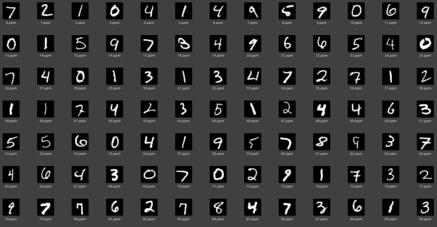
All that is left is to prepare the program for a parallel execution on multiple devices. Firstly we’ll download the 10 000 testing images and then transform the first 100 images into ppms (we can use the functions that are already used):
char filename[50];
for (int i = 0; i < 100; i++) {
    sprintf(filename, "%d.ppm", i);
    toPPM(filename, img[i], 28, 28);
}
We will pack the digits in a zip file along with network.json which I will name tasks.zip. Next up we’ll change the main function so it can accept command line arguments (these will specify which files to read).
int main(int argc, char* argv[]) {
    int start_index;
    if (argc > 1) {
        start_index = atoi(argv[1]);
        printf("The integer value is: %d\n", start_index);
    } else {
        return 1;
    }

    int numImg = 10;
    int imgSize = 28*28;
    unsigned char** img = load_ppm(start_index, numImg, imgSize);


    network *homeNN = (network*)malloc(sizeof(network));
    import_network_from_json("network.json", homeNN);
    printf("Import done!\n");

    float input[28 * 28];
    for (int i = 0; i < 10; i++) {
        for (int j = 0; j < 28 * 28; j++) {
            input[j] = (float)img[i][j] / 255.0;
        }
        int prediction = predict(homeNN, input);
        printf("File %d.ppm was classified as: %d\n", i+start_index, prediction);
    }


    free_architecture(homeNN);
    for (int i = 0; i < numImg; i++) {
        free(img[i]);
    }
    free(img);

    return 0;
}
What this does is that the argument that is provided to the programme call will determine the starting index of a batch of images that will be classified. The conversion from ppm looks like this:
unsigned char** load_ppm(int start_index, int numImg, int imgSize) {
    char filename[50];
    unsigned char** img = (unsigned char**)malloc(numImg * sizeof(unsigned char*));
    if (img == NULL) {
        printf("Memory allocation failed\n");
        return NULL;
    }

    for (int i = 0; i < numImg; i++) {
        sprintf(filename, "%d.ppm", i + start_index);
        FILE* file = fopen(filename, "rb");
        if (!file) {
            printf("Couldn't open %s\n", filename);
            return NULL;
        }

        char format[3];
        int width, height, maxVal;

        fscanf(file, "%2s", format);
        if (format[0] != 'P' || format[1] != '3') {
            printf("Format ERROR\n");
            fclose(file);
            return NULL;
        }
        fscanf(file, "%d %d", &width, &height);
        if (width != height || width * height != imgSize) {
            printf("Size ERROR\n");
            fclose(file);
            return NULL;
        }
        fscanf(file, "%d", &maxVal);
        if (maxVal != 255) {
            printf("Maximum value ERROR\n");
            fclose(file);
            return NULL;
        }

        img[i] = (unsigned char*)malloc(imgSize * sizeof(unsigned char));
        if (img[i] == NULL) {
            printf("Memory allocation failed for image %d\n", i);
            fclose(file);
            return NULL;
        }

        for (int j = 0; j < imgSize; j++) {
            int r, g, b;
            fscanf(file, "%d %d %d", &r, &g, &b);
            img[i][j] = (unsigned char)r;
        }

        fclose(file);
    }

    return img;
}
I prepared the client.json file with the following contents:
{
  "parent": {
    "binary": { "ref": "client.wasm" },
    "rootfs": { "ref": "tasks.zip" }
  },
  "tasks": [
    {
      "args": ["client.wasm", "0"]
    },
    {
      "args": ["client.wasm", "10"]
    },
    {
      "args": ["client.wasm", "20"]
    },
    {
      "args": ["client.wasm", "30"]
    },
    {
      "args": ["client.wasm", "40"]
    },
    {
      "args": ["client.wasm", "50"]
    },
    {
      "args": ["client.wasm", "60"]
    },
    {
      "args": ["client.wasm", "70"]
    },
    {
      "args": ["client.wasm", "80"]
    },
    {
      "args": ["client.wasm", "90"]
    }
  ]
}
These 10 tasks will be divided among the available providers connected to the Wasimoff network. So to recap I had to prepare the following on the client side:
├── client.json
├── tasks.zip
│   ├── network.json
│   └── the images (in ppm format)
├── client.wasm
Results#
I decided to use my main laptop into a broker and a client, while my old Lubuntu laptop, tablet, Raspberry Pi and Fairphone would be providers - each provider would offer one worker, so the tasks would be evenly distributed. I uploaded all the files on my PC and started the client.json:

After a short while I got the results!
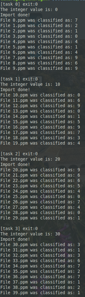
Hurray 🥳, the distributed neural network works as it should!
By the way here are two numbers that were classified incorrectly among the first 40:


The left one was classified as a 6 (which to be honest is a reasonable guess) and the right one was also classified as a 6, even though it’s a very ugly 4. So the network works pretty well as long as the digits don’t get too wonky.
The results are very promising. In case one needs to perform some sort of classification with a small embedded neural network, it should be possible to parallelise the computation close to the edge by offloading the classification to more powerful devices like Raspberry Pis with very high flexibility, because the tasks can easily be offloaded to any device that can run web browsers no matter the hardware - Wasimoff might prove to be an embedded edge computing beast
Sources#
- Using neural nets to recognize handwritten digits by Michael Nielsen, chapter 1 and 2: http://neuralnetworksanddeeplearning.com/chap1.html
- Fabian Pallasidies, Sven Goedke et al, From single neurons to behavior in the jellyfish Aurelia aurita: https://elifesciences.org/articles/50084
- Mayur Bhole: Building Neural Network Framework in C using Backpropagation: https://medium.com/analytics-vidhya/building-neural-network-framework-in-c-using-backpropagation-8ad589a0752d
- Konrad Gajdus: From Theory to Code: Implementing a Neural Network in 200 Lines of C: https://konrad.gg/blog/posts/neural-networkin-in-200-lines-of-c.html